Images with low contrast may be enhanced by manipulating its histogram. This post on my blog will show you just that.
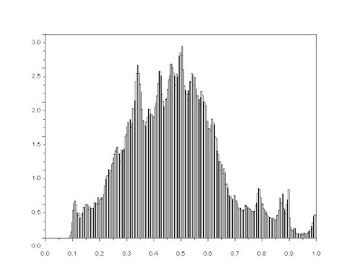
(Histogram is a graph showing how many pixels have a particular value, from 0-255, in a grayscale image. This is equal to the probability distribution function or PDF.)
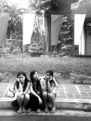
Start with an image that you want to enhance:
(Histogram is a graph showing how many pixels have a particular value, from 0-255, in a grayscale image. This is equal to the probability distribution function or PDF.)
Start with an image that you want to enhance:
 Figure 1: original image
Convert this image into grayscale:
 Figure 3: Normalized histogram of the grayscale image
From the obtained histogram, get the CDF(cumulative probability function) using the scilab fuction cumsum():
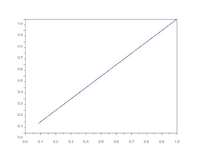
 Figure 5: Desired CDF
By pixel-per-pixel backprojection, the undesired pixels may be replaced with the x-values of the desired CDF. The image below shows the modified image. If compared with the original image, this one is clearer and more resolved.
 Figure 6: Processed image by backprojection
Other softwares such as photoshop and GIMP allows you to "twick" your image's histogram. As a comparison, I also tried manipulating my original image's histogram in imagej. The results are shown below:
Using imagej:
 Figure 8: Processed image by manipulating histogram using imagej
CODE:
//reading the image
I = gray_imread('C:\Users\cindyleen\Desktop\DSC03137.jpg');
scf();
//imshow(I);
//PLOTTING THE HISTOGRAM OF THE IMAGE
histplot(256,I);
//TABULATION OF FREQUENCY PER GRAYSCALE VALUE(0-256)
tab = tabul(I, 'i');
x = tab(:,1);
y = tab(:,2)/sum(tab(:,2)); //normalization of frequency
//disp(sum(y))
//scf();
//plot(x, y, '.')
//getting the CDF
ycum = cumsum(y);
scf();
plot(x, ycum) //this is the CDF of your image
//desired CDF(linear)
scf();
plot(x,x)
//BACKPROJECTION
[r c] = size(I);
ix = I(:);
yp = interp1(x,ycum,ix);
xd = interp1(x,x,yp,['spline']);
//displaying the processed image
Inew = matrix(xd, [r c]);
scf();
imshow(Inew);
I would to give my self a grade of 9.5 for this activity. Although I did manage to get all output ask, I'm afraid I wasn't able to explain the method clearly in this blog.
Thank you Joseph for all the help in this activity! :D


No comments:
Post a Comment