A6 - Fourier Transform Model of Image Formation

This activity is an introduction to Fourier Transform (FT). If you're a Physics major then you might already be familiar with it but quite honestly, seeing how FT works visually gains you so much more understanding of this transformation.

First, let's see the equation for FT of a 2D data such as an image:

Basically what this equation tells us is that given an image in spatial domain, the FT of it will be the image in frequency domain (X -> 1/X and Y->1/Y).

FT is so widely used that programming softwares such as Matlab and Scilab already have functions for them. :)

The objective of this activity is for us to familiarize ourselves with the basics of FT using Scilab.

A6.A: Familiarization w/ discrete FFT

First, an image (128x128) of a white circle on black background is obtained. I did mine in GIMP but other softwares may also be used like paint and photoshop.

Figure 1: White Circle in Black Background

Next, the image of the circle (as shown in figure 1) is opened in as a grayscale image using the functions: imread() and im2gray() or you can just use im2gray(imread('your image'))

Applying the function fft2() (for a 2D data such as an image) on the image will give you the image below:

Figure 2: FFT of Circle

As you can see in figure 2, the areas of interest are located on the corners of the image. This is because when applying fft(), the quadrants interchange. To arrange the quadrants such as it is the same as in the original image, the function fftshift() is used. The figure below shows the shifted image. We are on the right track since this is what we expect the Fourier Transfrom of a cicle would look like. :D

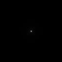Figure 3: Shifted FFT of Circle

Applying another fft2() to the already fftied image will result back to our original image.

Figure 4: Inverse FFT of the FFT of Circle

The figures below are the results when you apply the fuctions: fft2() -> fftshift() -> fft2() on an image of letter "A" instead of a circle:

Figure 5: White Letter "A" in Black Background

Figure 6: FFT of the Letter "A"

Figure 7: Shifted FFT of the Letter "A"

Figure 8: Inverse FFT of the FFT of Letter "A"

As illustated in figure 8, when you fft an already fftied image, you'll actually end up with an inverted image of the original image. We would have not noticed this if only symmetric shapes are used such as a circle.

Code:

//CIRCLE
//no.2
I = im2gray(imread('C:\Users\cindyleen\Desktop\circle.bmp'));

//no.3
FT = fft2(I);
AFT = abs(FT);
scf(); imshow(AFT, []);
AFTn = (AFT - min(AFT))/(max(AFT)-min(AFT));
imwrite(AFTn, 'C:\Users\cindyleen\Desktop\no3circlenorm.bmp');

//no.4
FTshift = fftshift(abs(FT));
scf(); imshow(FTshift, []);
FTshiftn = (FTshift - min(FTshift))/(max(FTshift)-min(FTshift));
imwrite(FTshiftn, 'C:\Users\cindyleen\Desktop\no4circlen.bmp');

//no.5
FFT = fft2(FT);
FFTabs = abs(FFT);
scf(); imshow(FFTabs, []);
FFTabsn = (FFTabs - min(FFTabs))/(max(FFTabs)-min(FFTabs));
imwrite(FFTabsn, 'C:\Users\cindyleen\Desktop\no5circlen.bmp');

//no.6
I = im2gray(imread('C:\Users\cindyleen\Desktop\A.bmp'));
FT = fft2(I);
AFT = abs(FT);
scf(); imshow(AFT, []);

AFTn = (AFT - min(AFT))/(max(AFT)-min(AFT));
imwrite(AFTn, 'C:\Users\cindyleen\Desktop\no3An.bmp');

FTshift = fftshift(abs(FT));
scf(); imshow(FTshift, []);

FTshiftn = (FTshift - min(FTshift))/(max(FTshift)-min(FTshift));
imwrite(FTshiftn, 'C:\Users\cindyleen\Desktop\no4An.bmp');

FFT = fft2(FT);
FFTabs = abs(FFT);
scf(); imshow(FFTabs, []);

FFTabsn = (FFTabs - min(FFTabs))/(max(FFTabs)-min(FFTabs));
imwrite(FFTabs, 'C:\Users\cindyleen\Desktop\no5An.bmp');

A6.B: Simulation of an Imaging Device

An image (128x128) of the letters "VIP" and circles varying in radius are created (this will serve as your aperture).

The fft of the VIP image and the fftshift of the circles are obtained.

After this, the fftied image of the VIP is convolved with each of the fftshifted images of circle.

The convolutin results are shown below:

Figure 9a: Convolution of "VIP" with circle of radius 0.1

Figure 9b: Convolution of "VIP" with circle of radius 0.2

Figure 9c: Convolution of "VIP" with circle of radius 0.4

Figure 9d: Convolution of "VIP" with circle of radius 0.6

Figure 9e: Convolution of "VIP" with circle of radius 0.8

We can see that as the radius of the aperture (circle) increase, the clearer or more crisp the convolution gets.

Code:

x = linspace(-1,1,128);
[X,Y] = meshgrid(x);
r = sqrt(X.^2 + Y.^2);
circle = zeros(size(X,1), size(X,2));
circle(find (r <=1.1)) = 1.0;
imshow(circle,[]);

r = im2gray(imread('C:\Users\cindyleen\Desktop\VIP.bmp'));
a = im2gray(circle);

Fr = fftshift(a);
Fa = fft2(r);
FRA = Fr.*(Fa);
IRA = fft2(FRA); //inverse FFT
FImage = abs(IRA);
FImagen = (FImage - min(FImage))/(max(FImage) - min(FImage));
imshow(FImage, [ ]);
imwrite(FImagen, 'C:\Users\cindyleen\Desktop\11r.bmp')

A6.C: Template Matching using Correlation

In this part of the activity we learned that template matching refers to a pattern recognition that enables us to find identical patterns.

Figure 10: An image with texts

Figure 11: An image of the letter "A"

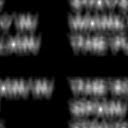Figure 12: Element per element multiplication of figure 10 and figure 11

Code:


words = im2gray(imread('C:\Users\cindyleen\Desktop\the rain.bmp'));
a = im2gray(imread('C:\Users\cindyleen\Desktop\a.bmp'));

fftw = fft2(words);
ffta = fft2(a);

product = ffta.*(conj(fftw));
inverse = fft2(product);
ainverse = abs(inverse);
scf(); imshow(ainverse, []);
ainversen = (ainverse - min(ainverse))/(max(ainverse)- min(ainverse));
imwrite(ainversen, 'C:\Users\cindyleen\Desktop\part3.bmp');

A6.D: Edge Detection using a Convolution Integral

Edge detection can be done by just performing a convolution (use scilab's imcorrcoef() function to do this) on the image you want to get edges from and a matrix pattern of an edge.

Here are the patterns used for this part of the activity:
1. [-1 -1 -1; 2 2 2; -1 -1 -1]
2. [-1 2 -1; -1 2 -1; -1 2 -1]
3. [-1 -1 -1; -1 8 -1; -1 -1 -1]
4. [2 -1 1; 1 2 -1; -1 1 2]
5. [-1 1 2; 1 2 -1; 2 -1 1]

The figures below are the results when I convolved an image of "VIP" to different edge detection patterns:

Figure 13a: VIP convolved w/ pattern 1

Figure 13b: VIP convolved w/ pattern 2

Figure 13c: VIP convolved w/ pattern 3

Figure 13d: VIP convolved w/ pattern 4

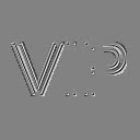Figure 13e: VIP convolved w/ pattern 5

It is clearly shown that using pattern no.3 (a Gaussian) yields the best results for edge detection.

Codes:

r = im2gray(imread('C:\Users\cindyleen\Desktop\vip and circle\VIP.bmp'));
pattern1 = [-1 -1 -1; 2 2 2; -1 -1 -1];
pattern2 = [-1 2 -1; -1 2 -1; -1 2 -1];
pattern3 = [-1 -1 -1; -1 8 -1; -1 -1 -1];
pattern4 = [2 -1 1; 1 2 -1; -1 1 2];
pattern5 = [-1 1 2; 1 2 -1; 2 -1 1];
conv = imcorrcoef(r, pattern5);
scf(); imshow(conv, []);

convn = (conv - min(conv))/(max(conv) - min(conv));
imwrite(convn, 'C:\Users\cindyleen\Desktop\5.bmp');

I think I would give myself a grade of 10 for this activity.

Thanks Joseph for the help. :D