A14 - Image Compression

In this activity, we will be performing image compression done by most image compression algorithms when saving to formats like JPEG etc.

An image of size MxM may be represented as a point in an M^2 dimensional space. However, representing the said image as a point in such a highly dimensional space would be computationally expensive. That's where PCA(Principal Components Analysis) comes in. With the use of PCA, we would be able to find a new coordinate system(having less dimensions) with basis(eigenvectors) for representing the image. The pca() function in scilab outputs the eigenvectors as well as their corresponding eigenvalues.

Most image compression algorithms uses PCA for reducing information storage. This is done by reconstructing the image using only the eigenvectors having the most significant eigenvalues.

Given the image:

Figure 1: Image to be compressed

Using PCA we would be able to compress this image using 100%, 98%, 95% and 90% of the total eigenvectors.

100%:

98%:

95%:

90%:

As illustrated, as lesser eigenvectors are used to represent the image, the more pixelated in gets. This is because as you decrese the number of eigenvectors, less information are stored per pixel.

I would like to give myself a grade of 9/10 for this activity. I was able to get the results for compressing an image using PCA. Less one point for not blogging it clearly.

A13 – Color Image Segmentation

In some cases, you may only want to select a particular portion on an image where you would be performing image processing. One way of selecting that said portion would be to use color cues. In this activity, we would learn how to select only a particular color(ROI - region of interest) in an image. This is done through color segmentation.

There are two types of image segmentation which we would be doing:

1. Parametric: where we would assume the ROI to have a Gaussian PDF in the r and g values and segment the whole image using this PDF.

2. Non-parametric segmentation: where we would obtain the 2D histogram of the ROI and use the this histogram to segment the image using histogram backprojection

where r and g are the normalized chromaticity coordinates given by:

r = R/R+G+B, g = G/R+G+B

recall:

Histogram backprojection: a technique where using the color histogram, a pixel location is given a value equal to its histogram value in chromaticity space. (see activity 8)

Given the image:

Figure 1: Image to be segmented

What I want to do is to just select the rose. (ROI = rose)

Parametric

Figure 2: Result using parametric color segmentation

White pixels represent the present of the cue color while black pixels represent absence of the cue color. Using parametric color segmentation, we were able to select most parts of the rose. :D

Non-parametric

First, we get the histogram of the ROI. This is basically the same as getting the histogram for a gray image except that this time, the plot would be 3D -1 dimension for each color band(RGB).

Figure 3: Histogram of ROI

Figure 4: Result using non-parametric color segmentation

If I am to compare the two results, I would say the parametric color segmentation is ideal for selecting object with parts having slightly different colors. While non-parametric color segmentation should be used for selecting a specific color.

I would like to give myself a grade of 9/10 for this activity. I was able to get the results asked for but failed to blog this activity in a more detailed way.

A11 – Playing Notes by Image Processing

Would it be just the coolest thing if you'd be able to play a song using just its music sheet and scilab? Well its possible! :D

In this activity, we will be playing notes in scilab using the image processing techniques we have learned so far.

The music sheet that I chose is Jingle Bells (I know..I know... I'm just so excited for Christmas. Aren't you?).

Figure 1: Music sheet of Jingle Bells

Given the music sheet above, we find the location of the notes (notes present: whole, half and quarter note) using the imcorrcoef() function.

These are the templates that I used:

These are the locations of the notes:

half notes:


found in 1st line of music sheet


found in 2nd line of music sheet


found in 3rd line of music sheet


whole notes:


found in 1st line of music sheet


found in 3rd line of music sheet

quarter notes:


found in 1st line of music sheet


found in 2nd line of music sheet


found in 3rd line of music sheet

With the use of correlation, we are able to locate the respective notes in the sub-images of the music sheet. The next thing to do would be to know the location of each note on the staff for us to identify its pitch.

For assigning the pitch of the notes we need the frequencies of each pitch:

C = 261.63 Hz;
D = 293.66 Hz;
E = 329.63 Hz;
G = 392.00 Hz;
F = 349.23 Hz;

and assign the time for which each note will be playing:

quarternote: 0.25 sec
halfnote: 0.5 sec
wholenote: 1 sec

.....


I would like to give my self a grade of 5/10 for this activity since I wasn't able to play the notes but was able to locate the notes in the music sheet. :(

Frequencies of the pitches came from this site:
http://www.phy.mtu.edu/~suits/notefreqs.html

other reference:
186 handouts for activity 11

A12 – Color Image Processing

Have you ever had your photo taken and you somehow appeared bluish or maybe orangish? You may find the photo "artsy" but do you ever wonder why this happens so? Its because digital cameras have settings called white balance. White balancing just refers to the transformations the camera does to make a white object in your image appear white. White balancing depends on the illumination condition under which the image was taken. That's why if you select an inappropriate white balance setting, your camera transforms the colors wrong.

I have taken an image of colorful objects under different white balance settings as shown below:

Figure 1: Image of colored objects taken under different white balance settings

Notice that using fluorescent and incandescent white balance settings makes your image appear bluish (especially using incandescent). From here we may say that using sunny(daylight) or cloudy are more appropriate white balance settings for this particular imaging conditions.

These are the two automatic white balancing algorithms that are available:

1. White patch algorithm: done by dividing the RGB channels of the image with the RGB components of the part of the image which should be white.

2. Gray world algorithm: white patch algorithm then averaging the RGB channels of the image.

These are the results using the two white balancing algorithms:

Figure 2: Results after performing white patch and gray world algorithm

Both algorithms worked with images quite well but I think that the gray world algorithm performed better since the white piece of paper looked more white upon its application.

The next part of the activity would be to apply both the white patch algorithm and the gray world algorithm on an image of objects having the same color.

Given this image:

Figure 3: Image of object having similar color
(sorry if the image is rotated...I couldn't figure out how to rotate this image)

Here are the results:

Figure 4: Result upon application of white patch algorithm

Figure 5: Result upon using gray world algorithm

Through visual inspection, I would say that using white patch algorithm yield better result than gray world algorithm since white patch algorithm captured the background color better (supposed to be green). This is probably because for the gray world algorithm to work optimally, sample colors from red, green and blue should be present. For this particular image however, only green colored objects are present.

I would like to give myself a grade of 10/10 for this activity since I was able to implement both algorithms and presented results asked.

A10 – Binary Operations

First part: Finding the cells of ordinary cells

In this activity we apply what we have learned about morphological operations (see activity 9) for finding the area of cells.

This operation can actually be easily done using opening and closing operations, however, these functions are not present in scilab. Lucky for us, the said functions can also be done using the erode() and dilate() functions.

Remember this:
Open = Erode + Dilate
Close = Dilate + Erode

The image below is an image model of cells:

Figure 1: Image of cells

We divide this image into 9 sub-images...

Figure 2: Collage of sub-images of original image

To separate the cells from the background, we look at its histogram:

Figure 3: Histogram of one sub-image

Since we know that the background have a gray color, using the appropriate values for im2bw() (near white), we would end up with the binarized image below:

Note: For illustration purposes, the thresholded image above is just one sub-image of the original image, however, all the operations in this activity are applied to all the sub-images.

After getting the thresholded image, we may now apply erosion and dilation operations to fill-up the cells and separate cells that are overlapping. The result after applying these operations is the image below:

Figure 4: Sub-image after erosion and dilation

As you can see, some cells are reduced to smaller sizes than the original while other cells are still not separated from each other(which may be interpreted as larger cells in a 2D image). Since our goal is to average the cell sizes(areas), it would be wrong to use these "reduced in size cells" and "large cells" for finding the mean area. To solve this problem, we look at the histogram of areas of all cells:

Figure 5: Histogram of cell areas

Using this histogram, we may assign a specific threshold locating the cells for which we would get the areas from.

To get the area of a cell, we just add the pixels comprising each cell. Repeat this for all cells and find the mean.

Results:
Mean area: 451.69231
Variance: 66.891858

Second part: Isolating cancer cells

In this part of the activity, our goal is to locate the cancer cells in the image below:

Figure 6: Image of cells with cancer

In this model image, the cancer cells are represented by the larger cells. Fortunately, none of them are overlapping with the normal cells making our work a lot easier.

Basically, the same steps are applied but this time several erosion operations are applied to separate the cells from each other.

Here are the result:

The cancer cells are successfully isolated from the normal cells.

I would like to give myself a grade of 10/10 since I was able to obtain the results asked for.

Thanks to Joseph for the help.

A9 – Morphological Operations

Predicted outcomes upon application of erosion and dilation operations:

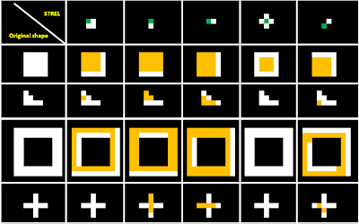
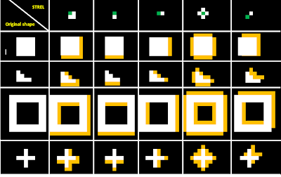
Before using scilab to simulate the results when we apply the erosion and dilation operations, we were first asked to predict what these results would be. I used Microsoft word to illustrate my predictions by putting gridlines and drawing squares as pixels.

Here are my predictions...

Figure 1: Predictions for erosion

NOTE: The resulting image is comprised ONLY of the yellow pixels. The white pixels are only included to illustrate how much of the original image are removed.

Figure 2: Predictions for dilation

NOTE: The resulting image is the combination of the yellow and white pixels.



Outcomes upon application of erosion and dilation operators using SCILAB:

EROSION:

Figure 3: Erosion using a 2x2 ones strel

Figure 4: Erosion using a 2x1 ones strel

Figure 5: Erosion using a 1x2 ones strel

Figure 6: Erosion using a cross (3x3) strel

Figure 7: Erosion using a diagonal (0 1; 1 0) strel

NOTE: Blank figure means that no pixel remained after the erosion operation.

DILATION:

Figure 8: Dilation using a 2x2 ones strel

Figure 9: Dilation using a 2x1 ones strel

Figure 10: Dilation using a 1x2 ones strel

Figure 11: Dilation using a cross (3x3) strel

Figure 12: Dilation using a diagonal (0 1; 1 0) strel

I'm glad to see that my predictions are correct! :D

Other morphological operators:

1. Thin: performs a thinning operation on binary objects

Figure 13: objects(left), objects after thinning operation(right)

2. Skel: another thinning operation where the output object can be further pruned by thresholding

below are examples of what your object will look like after skel operation:

Figure 14: objects(left), objects after skel operation(right)

CODE:

stacksize(1000000);

o1 = zeros(11,11);
o1(4:8,4:8) = 1
//imshow(o1,[])

o2 = zeros(8,8);
o2(4,3) = 1;
o2(5,3:4) = 1;
o2(6,3:6) = 1;
//imshow(o2,[])


o3 = zeros(14,14);
o3(3:12,3:12) = 1;
o3(5:10,5:10) = 0;
//imshow(o3,[])


o4 = zeros(9,9);
o4(3:7,5) = 1;
o4(5,3:7) = 1;
//imshow(o4,[])

//Structuring elements
a = [1 1; 1 1];
b = [1; 1];
c = [1 1];
d = [0 1 0; 1 1 1; 0 1 0]
e = [0 1; 1 0]

////////////////////////////////////////////////////////////////

//erode

a1 = erode(o1, a, [1,1]);
a2 = erode(o2, a, [1,1]);
a3 = erode(o3, a, [1,1]);
a4 = erode(o4, a, [1,1]);

subplot(1, 4, 1);imshow(a1, []);
subplot(1, 4, 2);imshow(a2, []);
subplot(1, 4, 3);imshow(a3, []);
subplot(1, 4, 4);imshow(a4, []);

b1 = erode(o1, b, [1,1]);
b2 = erode(o2, b, [1,1]);
b3 = erode(o3, b, [1,1]);
b4 = erode(o4, b, [1,1]);

subplot(1, 4, 1);imshow(b1, []);
subplot(1, 4, 2);imshow(b2, []);
subplot(1, 4, 3);imshow(b3, []);
subplot(1, 4, 4);imshow(b4, []);

c1 = erode(o1, c, [1,1]);
c2 = erode(o2, c, [1,1]);
c3 = erode(o3, c, [1,1]);
c4 = erode(o4, c, [1,1]);

subplot(1, 4, 1);imshow(c1, []);
subplot(1, 4, 2);imshow(c2, []);
subplot(1, 4, 3);imshow(c3, []);
subplot(1, 4, 4);imshow(c4, []);

d1 = erode(o1, d, [2,2]);
d2 = erode(o2, d, [2,2]);
d3 = erode(o3, d, [2,2]);
d4 = erode(o4, d, [2,2]);

subplot(1, 4, 1);imshow(d1, []);
subplot(1, 4, 2);imshow(d2, []);
subplot(1, 4, 3);imshow(d3, []);
subplot(1, 4, 4);imshow(d4, []);

e1 = erode(o1, e, [2,1]);
e2 = erode(o2, e, [2,1]);
e3 = erode(o3, e, [2,1]);
e4 = erode(o4, e, [2,1]);

subplot(1, 4, 1);imshow(e1, []);
subplot(1, 4, 2);imshow(e2, []);
subplot(1, 4, 3);imshow(e3, []);
subplot(1, 4, 4);imshow(e4, []);

/////////////////////////////////////////////////////////

//dilate

a1 = dilate(o1, a, [1,1]);
a2 = dilate(o2, a, [1,1]);
a3 = dilate(o3, a, [1,1]);
a4 = dilate(o4, a, [1,1]);

subplot(1, 4, 1);imshow(a1, []);
subplot(1, 4, 2);imshow(a2, []);
subplot(1, 4, 3);imshow(a3, []);
subplot(1, 4, 4);imshow(a4, []);

b1 = dilate(o1, b, [1,1]);
b2 = dilate(o2, b, [1,1]);
b3 = dilate(o3, b, [1,1]);
b4 = dilate(o4, b, [1,1]);

subplot(1, 4, 1);imshow(b1, []);
subplot(1, 4, 2);imshow(b2, []);
subplot(1, 4, 3);imshow(b3, []);
subplot(1, 4, 4);imshow(b4, []);

c1 = dilate(o1, c, [1,1]);
c2 = dilate(o2, c, [1,1]);
c3 = dilate(o3, c, [1,1]);
c4 = dilate(o4, c, [1,1]);

subplot(1, 4, 1);imshow(c1, []);
subplot(1, 4, 2);imshow(c2, []);
subplot(1, 4, 3);imshow(c3, []);
subplot(1, 4, 4);imshow(c4, []);

d1 = dilate(o1, d, [2,2]);
d2 = dilate(o2, d, [2,2]);
d3 = dilate(o3, d, [2,2]);
d4 = dilate(o4, d, [2,2]);

subplot(1, 4, 1);imshow(d1, []);
subplot(1, 4, 2);imshow(d2, []);
subplot(1, 4, 3);imshow(d3, []);
subplot(1, 4, 4);imshow(d4, []);

e1 = dilate(o1, e, [2,1]);
e2 = dilate(o2, e, [2,1]);
e3 = dilate(o3, e, [2,1]);
e4 = dilate(o4, e, [2,1]);

subplot(1, 4, 1);imshow(e1, []);
subplot(1, 4, 2);imshow(e2, []);
subplot(1, 4, 3);imshow(e3, []);
subplot(1, 4, 4);imshow(e4, []);

I would like to give my self a grade of 10/10 for this activity since I was able to achieve the desired results.

Thanks to Joseph and Dane for helping me with this activity!

Thanks to BA for keeping me company while finishing this activity. :P

references:
1. 187 activity 9 handout
2. http://homepages.inf.ed.ac.uk/rbf/HIPR2/skeleton.htm