A8.A - Convolution Theorem

Activity 8 is a 3 part activity. This first one is a continuation of activity 7. In here we are still familiarizing with the FFTs of different functions.


1) Dirac delta:

(a) (b)

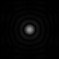
Figure 1: 2 dirac delta(a), its FFT(b)

- the FFT of two dirac deltas is a periodic function along the direction of the dirac deltas

2. Circles with different radii:

(a) (b)

Figure 2: 2 circles w/ radius = 6px (a), FFT(b)

(a) (b)

Figure 3: 2 circles w/ radius = 10px (a), FFT(b)

(a) (b)

Figure 4: 2 circles w/ radius = 15px (a), FFT(b)

- the FFT of a two circles come out as an airy disk
- it is observed that as the diameter of the circles get bigger, the airy disk diameter of its FFT becomes smaller

3. Squares with different lengths:

(a) (b)

Figure 5: 2 squares w/ width = 6px (a), FFT(b)

(a) (b)

Figure 6: 2 square w/ width = 10px (a), FFT(b)

(a) (b)

Figure 7: 2 square w/ width = 15px (a), FFT(b)

- the FFT of two squares is are square patterns along the x and y axis (or rather fx and fy axis), kind of like a diffraction pattern, that reduces size as it becomes farther and farther from the origin
- just like in the circle, as the length of the squares increase, its FFT pattern gets smaller/thinner

4. Gaussian:

Figure 8: two Gaussian

(a) (b) (c)

Figure 9: FFts of Gaussian w/ different radii (increasing variance)

- same trend arise, as in the two circles and two squares, we can see that as the variance of the Gaussians becomes larger, their FFTs become smaller

5. Random Pattern

Figure 10: A random pattern

patterns used:

pattern1 = [-1 -1 -1; 2 2 2; -1 -1 -1];
pattern2 = [-1 2 -1; -1 2 -1; -1 2 -1];
pattern3 = [-1 -1 -1; -1 8 -1; -1 -1 -1];
pattern4 = [2 -1 1; 1 2 -1; -1 1 2];
pattern5 = [-1 1 2; 1 2 -1; 2 -1 1];

function used: imconv(a, b)
-basically, this function just repeats whatever pattern you have (pattern b) in the points of pattern a

Figure 11: Convolution w/ pattern 1

Figure 12: Convolution w/ pattern 2

Figure 13: Convolution w/ pattern 3

Figure 14: Convolution w/ pattern 4

Figure 15: Convolution w/ pattern 5

7. Equally Distributed Pattern

Figure 16: pattern with equally distributed white pixels, distance = 10 px (a), its FFT (b)

- the FFT are also points but as the distance between the white pixels of input data (a) increases, the distance between the points in the FFT decreases


CODE:

//8A

//no.1

I = im2gray(imread('C:\Users\cindyleen\Desktop\1st sem classes\186\a8\dots.bmp'));
fftI = fft2(I);
absI = abs(fftI);
//absIn = (absI - min(absI))/(max(absI)-min(absI));

imwrite(absI, 'C:\Users\cindyleen\Desktop\1st sem classes\186\a8\8Ano1.bmp');

//no.2

I = im2gray(imread('C:\Users\cindyleen\Desktop\1st sem classes\186\a8\r=30px.bmp'));
fftI = fft2(I);
absI = fftshift(abs(fftI));
absIn = (absI - min(absI))/(max(absI)-min(absI));
imshow(absIn);

imwrite(absIn, 'C:\Users\cindyleen\Desktop\1st sem classes\186\a8\8Ano2c.bmp');

//no.3

I = im2gray(imread('C:\Users\cindyleen\Desktop\1st sem classes\186\a8\l=30px.bmp'));
fftI = fft2(I);
absI = fftshift(abs(fftI));
absIn = (absI - min(absI))/(max(absI)-min(absI));
imshow(absIn);

imwrite(absIn, 'C:\Users\cindyleen\Desktop\1st sem classes\186\a8\8Ano3c.bmp');

//no.5

//gaussian
var = 0.3;
N = 256;
x = linspace(-10, 10, N);
[X Y] = meshgrid(x);
cent = 5;
g = exp(-((X-cent).^2 + Y.^2)./var) + exp(-((X+cent).^2 + Y.^2)./var);
ng = (g - min(g))./(max(g) - min(g));
imshow(ng, [])
//imwrite(ng, 'C:\Users\cindyleen\Desktop\1st sem classes\186\a8\gaussian.bmp');

fg = abs(fftshift(fft2(g)));
nfg = (fg- min(fg))./(max(fg) - min(fg));
imwrite(nfg, 'C:\Users\cindyleen\Desktop\1st sem classes\186\a8\8Ano5c(var=0.3).bmp');

//no.6

I = im2gray(imread('C:\Users\cindyleen\Desktop\1st sem classes\186\a8\random.bmp'));
pattern1 = [-1 -1 -1; 2 2 2; -1 -1 -1];
pattern2 = [-1 2 -1; -1 2 -1; -1 2 -1];
pattern3 = [-1 -1 -1; -1 8 -1; -1 -1 -1];
pattern4 = [2 -1 1; 1 2 -1; -1 1 2];
pattern5 = [-1 1 2; 1 2 -1; 2 -1 1];
conv = imconv(I, pattern2);
imshow(conv);
imwrite(conv, 'C:\Users\cindyleen\Desktop\1st sem classes\186\a8\8Ano6b.bmp');

//no.7

I = im2gray(imread('C:\Users\cindyleen\Desktop\1st sem classes\186\a8\arranged1.bmp'));
fftI = fft2(I);
absI = abs(fftI);
absIn = (absI - min(absI))/(max(absI)-min(absI));
imshow(absIn);

I = im2gray(imread('C:\Users\cindyleen\Desktop\1st sem classes\186\a8\arranged2.bmp'));
fftI = fft2(I);
absI = abs(fftI);
absIn = (absI - min(absI))/(max(absI)-min(absI));
imshow(absIn);



I would like to give myself a grade of 10 for this activity.

thanks to joseph for never being tired of answering my questions. :D