A8.B - Fingerprints : Ridge Enhancement

In this part we will attempt to enhance a finger print from what we have learned about the Fourier Transforms(FT) of 2D patterns.

Given a fingerprint pattern...

Figure 1: Finger print pattern
from: ref:www.vosizneias.com/.../2009/02/fingerprint.jpg

We take its FT...

Figure 2: FT of finger print pattern

Question: How do we know which part of the FT we need and which are the parts we need to get rid of?

Answer: From what we have learned from past activities, we know that the FT of a periodic pattern is a pair of dirac deltas. Since our image is a finger print pattern, we can see that the periodic pattern is along every direction. From here we can conclude that the ring like structure at the center is the part of the FT that we want to retain. :D and ofcourse the center pixel since this corresponds to the background of the image.

I have chosen a Gaussian filter to select the part of the FT I want to retain...

Figure 3: A Gaussian Filter

Multiply the FT of the fingerprint pattern with the Gaussian filter I have created, leaving only the ring-like shape at the center and the background (center of the FT).

Figure 4: FT multiplied by the filter

Taking the inverse of Figure 4 results to the figure below. This is an enhanced fingerprint pattern...

Figure 5: Enhanced finger print pattern

CODE:

I = imread('C:\Users\cindyleen\Desktop\1st sem classes\186\a8\8b\fingerprint.jpg');
ffti = fft2(I);
li = log(abs(fftshift(ffti)));
ni = (li - min(li))/(max(li) - min(li));
//imshow(ni, []);
imwrite(ni, 'C:\Users\cindyleen\Desktop\fftfingerprint.bmp');

//gaussian filter
var1 = 0.1;
var2 = 1;
var3 = 7;
[a b] = size(ni);
x = linspace(-10, 10, b);
y = linspace(-10, 10, a);
[X Y] = meshgrid(x, y);
g = exp(-(X.^2 + Y.^2)./var1)-(exp(-(X.^2 + Y.^2)./var2)) + (exp(-(X.^2 + Y.^2)./var3));
ng = (g - min(g))./(max(g) - min(g));
//imshow(ng, []);
imwrite(ng, 'C:\Users\cindyleen\Desktop\filter.bmp');

mi = ffti.*fftshift(ng);
mi2 = ni.*ng;
mn = (mi2 - min(mi2))/(max(mi2) - min(mi2));
imshow(mi2, []);
imwrite(mn, 'C:\Users\cindyleen\Desktop\filterfft.bmp');

//take the fft

invft = abs(fft(mi));
in = (invft - min(invft))/(max(invft) - min(invft));
imshow(invft, []);
imwrite(in, 'C:\Users\cindyleen\Desktop\filter.bmp');

Grade: 10/10
Thanks Rap-rap!

A8.A - Convolution Theorem

Activity 8 is a 3 part activity. This first one is a continuation of activity 7. In here we are still familiarizing with the FFTs of different functions.


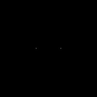
1) Dirac delta:

(a) (b)

Figure 1: 2 dirac delta(a), its FFT(b)

- the FFT of two dirac deltas is a periodic function along the direction of the dirac deltas

2. Circles with different radii:

(a) (b)

Figure 2: 2 circles w/ radius = 6px (a), FFT(b)

(a) (b)

Figure 3: 2 circles w/ radius = 10px (a), FFT(b)

(a) (b)

Figure 4: 2 circles w/ radius = 15px (a), FFT(b)

- the FFT of a two circles come out as an airy disk
- it is observed that as the diameter of the circles get bigger, the airy disk diameter of its FFT becomes smaller

3. Squares with different lengths:

(a) (b)

Figure 5: 2 squares w/ width = 6px (a), FFT(b)

(a) (b)

Figure 6: 2 square w/ width = 10px (a), FFT(b)

(a) (b)

Figure 7: 2 square w/ width = 15px (a), FFT(b)

- the FFT of two squares is are square patterns along the x and y axis (or rather fx and fy axis), kind of like a diffraction pattern, that reduces size as it becomes farther and farther from the origin
- just like in the circle, as the length of the squares increase, its FFT pattern gets smaller/thinner

4. Gaussian:

Figure 8: two Gaussian

(a) (b) (c)

Figure 9: FFts of Gaussian w/ different radii (increasing variance)

- same trend arise, as in the two circles and two squares, we can see that as the variance of the Gaussians becomes larger, their FFTs become smaller

5. Random Pattern

Figure 10: A random pattern

patterns used:

pattern1 = [-1 -1 -1; 2 2 2; -1 -1 -1];
pattern2 = [-1 2 -1; -1 2 -1; -1 2 -1];
pattern3 = [-1 -1 -1; -1 8 -1; -1 -1 -1];
pattern4 = [2 -1 1; 1 2 -1; -1 1 2];
pattern5 = [-1 1 2; 1 2 -1; 2 -1 1];

function used: imconv(a, b)
-basically, this function just repeats whatever pattern you have (pattern b) in the points of pattern a

Figure 11: Convolution w/ pattern 1

Figure 12: Convolution w/ pattern 2

Figure 13: Convolution w/ pattern 3

Figure 14: Convolution w/ pattern 4

Figure 15: Convolution w/ pattern 5

7. Equally Distributed Pattern

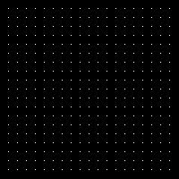
Figure 16: pattern with equally distributed white pixels, distance = 10 px (a), its FFT (b)

- the FFT are also points but as the distance between the white pixels of input data (a) increases, the distance between the points in the FFT decreases


CODE:

//8A

//no.1

I = im2gray(imread('C:\Users\cindyleen\Desktop\1st sem classes\186\a8\dots.bmp'));
fftI = fft2(I);
absI = abs(fftI);
//absIn = (absI - min(absI))/(max(absI)-min(absI));

imwrite(absI, 'C:\Users\cindyleen\Desktop\1st sem classes\186\a8\8Ano1.bmp');

//no.2

I = im2gray(imread('C:\Users\cindyleen\Desktop\1st sem classes\186\a8\r=30px.bmp'));
fftI = fft2(I);
absI = fftshift(abs(fftI));
absIn = (absI - min(absI))/(max(absI)-min(absI));
imshow(absIn);

imwrite(absIn, 'C:\Users\cindyleen\Desktop\1st sem classes\186\a8\8Ano2c.bmp');

//no.3

I = im2gray(imread('C:\Users\cindyleen\Desktop\1st sem classes\186\a8\l=30px.bmp'));
fftI = fft2(I);
absI = fftshift(abs(fftI));
absIn = (absI - min(absI))/(max(absI)-min(absI));
imshow(absIn);

imwrite(absIn, 'C:\Users\cindyleen\Desktop\1st sem classes\186\a8\8Ano3c.bmp');

//no.5

//gaussian
var = 0.3;
N = 256;
x = linspace(-10, 10, N);
[X Y] = meshgrid(x);
cent = 5;
g = exp(-((X-cent).^2 + Y.^2)./var) + exp(-((X+cent).^2 + Y.^2)./var);
ng = (g - min(g))./(max(g) - min(g));
imshow(ng, [])
//imwrite(ng, 'C:\Users\cindyleen\Desktop\1st sem classes\186\a8\gaussian.bmp');

fg = abs(fftshift(fft2(g)));
nfg = (fg- min(fg))./(max(fg) - min(fg));
imwrite(nfg, 'C:\Users\cindyleen\Desktop\1st sem classes\186\a8\8Ano5c(var=0.3).bmp');

//no.6

I = im2gray(imread('C:\Users\cindyleen\Desktop\1st sem classes\186\a8\random.bmp'));
pattern1 = [-1 -1 -1; 2 2 2; -1 -1 -1];
pattern2 = [-1 2 -1; -1 2 -1; -1 2 -1];
pattern3 = [-1 -1 -1; -1 8 -1; -1 -1 -1];
pattern4 = [2 -1 1; 1 2 -1; -1 1 2];
pattern5 = [-1 1 2; 1 2 -1; 2 -1 1];
conv = imconv(I, pattern2);
imshow(conv);
imwrite(conv, 'C:\Users\cindyleen\Desktop\1st sem classes\186\a8\8Ano6b.bmp');

//no.7

I = im2gray(imread('C:\Users\cindyleen\Desktop\1st sem classes\186\a8\arranged1.bmp'));
fftI = fft2(I);
absI = abs(fftI);
absIn = (absI - min(absI))/(max(absI)-min(absI));
imshow(absIn);

I = im2gray(imread('C:\Users\cindyleen\Desktop\1st sem classes\186\a8\arranged2.bmp'));
fftI = fft2(I);
absI = abs(fftI);
absIn = (absI - min(absI))/(max(absI)-min(absI));
imshow(absIn);



I would like to give myself a grade of 10 for this activity.

thanks to joseph for never being tired of answering my questions. :D

A7 - Properties of the 2D Fourier Transform

The journey of mastering Fourier Transform continues...

7.A Familiarization with FT of different 2D patterns

In this part of the activity we applied FT to some 2D patterns, namely: square, donut, annular square, slits and two dots. These FTs will be very handy in the next activities so be sure to remember them...

(a) - (b)

Figure 1: Square pattern (a), FT (b)

- The FT of a square looks like a diffraction pattern with the brightest spot at the center. The intensity is constantly decreasing as the pattern becomes farther from the center.

(a) - (b)
Figure 2: Annular 2D pattern (a), FT (b)

- The FT of an annular pattern is an Airy disk having amplitude not constantly decreasing as it becomes farther from the center. This is due to the presence of the annulus within the circle. Its FT interferes with that of the FT of the circle taken alone.

(a) - (b)
Figure 3: Square annulus pattern (a), FT (b)

- The FT is more or less similar to the FT of the square earlier. The only difference is that just like in the FT of a donut, the FT of the annulus inside interferes with that of the square alone. the result is an uneven distribution of intensity as you move farther away from the center -not constantly decreasing.

(a) - (b)

Figure 4: 2 slits symmetric along the x-axis (a), FT (b)

- I feel like I don't have to explain this figure anymore... :) From what we have learned from our earlier physics, the pattern produced when you shine light to two slits is an interference pattern. Suppose you have an experiment, let's say Young's double slit experiment, you can find the actual frequencies by just taking the FT of the sinusoidal pattern that you obtain.

(a)-(b)
Figure 5: 2 dots (a) FT (b)

- The FT of two slits symmetric about the x-axis looks a lot like a magnified airy pattern but multiply with a periodic pattern.

7.B: Anamorphic property of the Fourier Transform

all about SINES

(a) - (b)

Figure 6: Sinusoidal pattern along the y-axis (a), FT (b)

- The FT of a sine pattern along the y-axis are two dirac deltas also symmetric along the y-axis.


The following figure will show you how the FT of a sinusoid pattern changes if you...

...Change the frequency:

Figure 7: FTs with varying frequency: 2, 4, 8, 10 respectively

...add a constant bias:

(a) - (b)
Figure 8: sine with a bias (a), FT (b)

...rotate the sine pattern:

(a) - (b)
Figure 9: rotated sine pattern (a), FT(b)

...add two sines(one symmetric along the x-axis and one symmetric along the y-axis):
looks like an egg carton right? :D

(a) - (b)
Figure 10: egg carton pattern (a), FT (b)

...add several rotated sines:

(a) - (b)
Figure 10: sum of several rotated sine patterns (a), FT (b)

- my prediction on this part of the activity is that pair-by-pair dirac deltas will arise along the direction of their respective sine pattern.


CODE:
/////////////////////////////////////////////////
//7.A

a = im2gray(imread('C:\Users\cindyleen\Desktop\square.bmp'));
b = im2gray(imread('C:\Users\cindyleen\Desktop\squarea.bmp'));
c = im2gray(imread('C:\Users\cindyleen\Desktop\circlea.bmp'));
d = im2gray(imread('C:\Users\cindyleen\Desktop\slits.bmp'));
e = im2gray(imread('C:\Users\cindyleen\Desktop\dots.bmp'));

afft = fftshift(abs(fft2(a)));
scf();
imshow(afft, []);
afftn = (afft - min(afft))/(max(afft) - min(afft));
imwrite(afftn, 'C:\Users\cindyleen\Desktop\fftsquaren.bmp');

bfft = fftshift(abs(fft2(b)));
scf();
imshow(bfft, []);
bfftn = (bfft - min(bfft))/(max(bfft) - min(bfft));
imwrite(bfftn, 'C:\Users\cindyleen\Desktop\fftsquarean.bmp');

cfft = fftshift(abs(fft2(c)));
scf();
imshow(cfft, []);
cfftn = (cfft - min(cfft))/(max(cfft) - min(cfft));
imwrite(cfftn, 'C:\Users\cindyleen\Desktop\fftcirclean.bmp');

dfft = fftshift(abs(fft2(d)));
scf();
imshow(dfft, []);
dfftn = (dfft - min(dfft))/(max(dfft) - min(dfft));
imwrite(dfftn, 'C:\Users\cindyleen\Desktop\fftslitsn.bmp');

efft = fftshift(abs(fft2(e)));
scf();
imshow(efft, []);
efftn = (efft - min(efft))/(max(efft) - min(efft));
imwrite(efftn, 'C:\Users\cindyleen\Desktop\fftdotsn.bmp');

//////////////////////////////////////////////////////////////

//7.B
//1.
nx = 100; ny = 100;
x = linspace(-1,1,nx);
y = linspace(-1,1,ny);
[X,Y] = ndgrid(x,y);
f = 4 //frequency – you may change this later.
z = sin(2*%pi*f*X);
zn = (z - min(z))/(max(z) - min(z));
imshow(zn,[]);
imwrite(zn, 'C:\Users\cindyleen\Desktop\sine4.bmp');

fftsine = fftshift(abs(fft(z)));
scf();
imshow(fftsine, []);
fftsinen = (fftsine - min(fftsine))/(max(fftsine) - min(fftsine));
imwrite(fftsinen, 'C:\Users\cindyleen\Desktop\fftsine6n.bmp');

//4.
nx = 100; ny = 100;
x = linspace(-1,1,nx);
y = linspace(-1,1,ny);
[X,Y] = ndgrid(x,y);
f1 = 4 //frequency – you may change this later.
f2 = 3
z = sin(2*%pi*f1*X) + cos(2*%pi*f2*X);
zn = (z - min(z))/(max(z) - min(z));
imshow(zn,[]);
imwrite(zn, 'C:\Users\cindyleen\Desktop\sineandbias.bmp');


fftsine = fftshift(abs(fft(z)));
scf();
imshow(fftsine, []);
fftsinen = (fftsine - min(fftsine))/(max(fftsine) - min(fftsine));
imwrite(fftsinen, 'C:\Users\cindyleen\Desktop\fftsinebias3n.bmp');

//5.
nx = 100; ny = 100;
x = linspace(-1,1,nx);
y = linspace(-1,1,ny);
[X,Y] = ndgrid(x,y);
f = 4 //frequency – you may change this later.
theta = 30;
z = sin(2*%pi*f*(Y*sin(theta) + X*cos(theta)));
zn = (z - min(z))/(max(z) - min(z));
imshow(zn,[]);
imwrite(zn, 'C:\Users\cindyleen\Desktop\siner.bmp');

fftsiner = fftshift(abs(fft(z)));
fftsinern = (fftsiner - min(fftsiner))/(max(fftsiner) - min(fftsiner));
imshow(fftsinern, []);
imwrite(fftsinern, 'C:\Users\cindyleen\Desktop\fftsinern.bmp');

//6.
nx = 100; ny = 100;
x = linspace(-1,1,nx);
y = linspace(-1,1,ny);
[X,Y] = ndgrid(x,y);
f = 4 //frequency – you may change this later.
z = sin(2*%pi*4*X).*sin(2*%pi*4*Y);
imshow(z,[]);
zn = (z - min(z))/(max(z) - min(z));
imwrite(zn, 'C:\Users\cindyleen\Desktop\eggcarton.bmp');

fftsinexy = fftshift(abs(fft(z)));
fftsinexyn = (fftsinexy - min(fftsinexy))/(max(fftsinexy) - min(fftsinexy));
scf(); imshow(fftsinexyn, []);
imwrite(fftsinexyn, 'C:\Users\cindyleen\Desktop\fftsinexyn.bmp');

//7.
nx = 100; ny = 100;
x = linspace(-1,1,nx);
y = linspace(-1,1,ny);
[X,Y] = ndgrid(x,y);
f = 4 //frequency – you may change this later.
theta = 30;
z = sin(2*%pi*4*X).*sin(2*%pi*4*Y).*sin(2*%pi*f*(Y*sin(theta) + X*cos(theta)));
zn = (z - min(z))/(max(z) - min(z));
imshow(zn , []);
imwrite(zn, 'C:\Users\cindyleen\Desktop\sinexyr30.bmp');

fftsinexyr = fftshift(abs(fft(z)));
scf();
imshow(fftsinexyr, []);
fftsinexyrn = (fftsinexyr - min(fftsinexyr))/(max(fftsinexyr) - min(fftsinexyr));
imwrite(fftsinexyrn, 'C:\Users\cindyleen\Desktop\fftsinexyrn2.bmp');


I want to give myself a grade of 10 for this activity.

Arigato Joseph!!! :D