A2 - Scilab Basics

Today, we were asked to construct different kinds of apertures. These apertures are very helpful in the field of imaging; they may be used to confirm the validity of algorithms, as filters and for stimulating optical phenomena.

The figures below are the resulting apertures together with the code(written in Scilab) used.

example:

centered circular aperture

code:

nx = 300; ny = 300; //defines the number of elements along x and y
x = linspace(-1,1,nx); //defines the range in x
y = linspace(-1,1,ny); //defines the range in y
[X,Y] = ndgrid(x,y); //creates two 2-D arrays of x and y coordinates
r= sqrt(X.^2 + Y.^2); //note element-per-element squaring of X and Y
A = zeros (nx,ny); //creates a matrix consisting of all zero elements
A (find(r<0.7)) style="color: rgb(102, 255, 153);">//shows the image

resulting aperture:

Figure 1: Centered Circular Aperture

EXERCISES:

1. Centered Square Aperture

code:

nx = 300; ny = 300;
x = linspace(-1,1,nx);
y = linspace(-1,1,ny);
height = 50; //assigns a particular no. to the variable height (to be used later in the code)
[X,Y] = ndgrid(x,y);
A = zeros (nx,ny);

A (nx/2-height:nx/2+height, ny/2-height:ny/2+height) = 1; //finds the center of the image and designates the value equal to 1 to the square formed by adding and subtracting the variable height to this center

imshow (A, []);

Figure 2: Centered Square Aperture

2. Sinusoid along the x-direction

code:

nx = 300; ny = 300;
x = linspace(-1,1,nx);
y = linspace(-1,1,ny);
frequency = 6*%pi; //assigns the frequency of the sine wave
[X,Y] = ndgrid(x,y);
A = sin(X.*frequency);
imshow (A, []);

Figure 3: Sinusoid along the x-direction

3. Grating along the x-direction

code:

nx = 300; ny = 300;
x = linspace(-1,1,nx);
y = linspace(-1,1,ny);
frequency = 8*%pi;
[X,Y] = ndgrid(x,y);
A = sin(X.*frequency);
bw = im2bw(A, 0.3); //binarizes the pixel values
imshow (bw, []);

Figure 4: Gratings along the x-axis

4. Annular Aperture

code:

x = 300; ny = 300;
x = linspace(-1,1,nx);
y = linspace(-1,1,ny);
[X,Y] = ndgrid(x,y);
r= sqrt(X.^2 + Y.^2);
A = zeros (nx,ny);
A (find(r<0.7))>

Figure 5: Annular Apperture

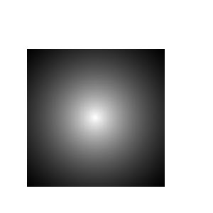
5. Circular aperture with graded transparency (gaussian transparency)

code:

nx = 300; ny = 300;
x = linspace(-1,1,nx);
y = linspace(-1,1,ny);
[X,Y] = ndgrid(x,y);
r= sqrt(X.^2 + Y.^2);
A = zeros (nx,ny);
A = exp(-r); //assigns an exponential value to radius r
imshow (A, []);

Figure 6: Circular aperture with graded transparency (gaussian transparency)

I would like to thank Joseph and Troy for helping me finish this activity... :)

encountered problems: familiarizing with scilab and blogging the results

Grade: 10/10 since I was able to produce the images which are asked for this activity.

Reference:
186 handout for activity 2